This page was generated from source/Jupyter/tutorials/tutorial-1-basic-plotting.ipynb. Interactive online version: Slideshow:

13.3.1. Basic plotting in Python

Here you will learn the basics of plotting in python including:

1. How to make a basic plot

2. How to add labels, legends and title to plot

3. How to change the color, fontsize, and other properties of the lines in the plot

4. How to save plots to files with different formats

Load the necessary packages

import numpy as np
import matplotlib.pyplot as plt

Let’s create some sample data to plot

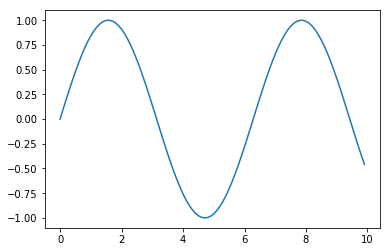
x=np.arange(0,10,.1)
y=np.sin(x)

A first quick plot:

plt.plot(x,y)

[<matplotlib.lines.Line2D at 0x1edf2412b70>]

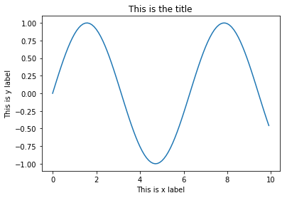
We want to add x and y labels and title to the plot:

plt.plot(x,y)
plt.xlabel('This is x label')
plt.ylabel('This is y label')
plt.title('This is the title')

Text(0.5, 1.0, 'This is the title')

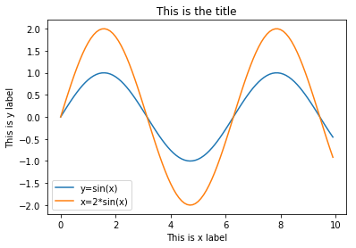
Now add more data (lines) to the plot, and make a legend

plt.plot(x,y,label='y=sin(x)')
plt.plot(x,2*y,label='x=2*sin(x)')
plt.xlabel('This is x label')
plt.ylabel('This is y label')
plt.title('This is the title')
plt.legend()

<matplotlib.legend.Legend at 0x1edf252db70>

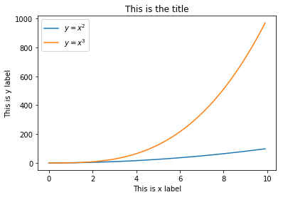
The mathematical formula can be improved in the legend

You need to use: $your formula here$

plt.plot(x,x*x,label='$y=x^2$')
plt.plot(x,x*x*x,label='$y=x^3$')
plt.xlabel('This is x label')
plt.ylabel('This is y label')
plt.title('This is the title')
plt.legend()

<matplotlib.legend.Legend at 0x1edf2597b70>

The superscript is made using ^{your superscript} and subscript is made using _{your subscript}

$x^{-3}$=\(x^{-3}\)

$x_{data}$=\(x_{data}\)

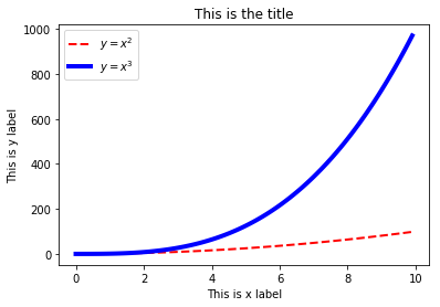
The line width, line style and line color can all be changed:

plt.plot(x,x*x,label='$y=x^2$',linewidth=2,color='r',linestyle='--')
plt.plot(x,x*x*x,label='$y=x^3$',linewidth=4,color='b')
plt.xlabel('This is x label')
plt.ylabel('This is y label')
plt.title('This is the title')
plt.legend()

<matplotlib.legend.Legend at 0x1edf262c048>

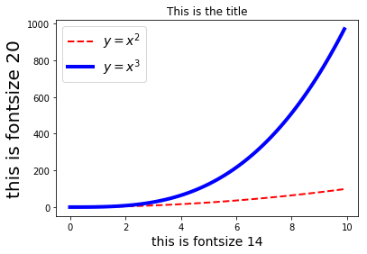
To change the text fontsize:

plt.plot(x,x*x,label='$y=x^2$',linewidth=2,color='r',linestyle='--')
plt.plot(x,x*x*x,label='$y=x^3$',linewidth=4,color='b')
plt.xlabel('this is fontsize 14',fontsize=14)
plt.ylabel('this is fontsize 20',fontsize=20)
plt.title('This is the title')
plt.legend(fontsize=14)

<matplotlib.legend.Legend at 0x1edf26c7128>

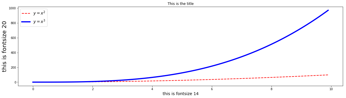
To change the figure size and shape:

plt.figure(figsize=(20,5))
plt.plot(x,x*x,label='$y=x^2$',linewidth=2,color='r',linestyle='--')
plt.plot(x,x*x*x,label='$y=x^3$',linewidth=4,color='b')
plt.xlabel('this is fontsize 14',fontsize=14)
plt.ylabel('this is fontsize 20',fontsize=20)
plt.title('This is the title')
plt.legend(fontsize=14)

<matplotlib.legend.Legend at 0x1edf276e160>

and finally, to save your figure to a file:

plt.figure(figsize=(20,5))
plt.plot(x,x*x,label='$y=x^2$',linewidth=2,color='r',linestyle='--')
plt.plot(x,x*x*x,label='$y=x^3$',linewidth=4,color='b')
plt.xlabel('this is fontsize 14',fontsize=14)
plt.ylabel('this is fontsize 20',fontsize=20)
plt.title('This is the title')
plt.legend(fontsize=14)
plt.savefig('sample.png',dpi=100)

You can use various formats such as jpg, pdf, etc.

You can control the quality of the saved file using dpi keyword. Be careful that using large numbers for dpi would make the process of saving figures slow and the created file very large.