This page was generated from source/Parameters/tutorials/param4-conductance.ipynb. Interactive online version: Slideshow:

10.3.4. Surface conductance parameters

from lmfit import Model, Parameters, Parameter
import numpy as np
import pandas as pd
from atmosp import calculate as ac
import numpy as np
from scipy.optimize import minimize
from pathlib import Path
import supy as sp
from sklearn.model_selection import train_test_split
import matplotlib.pyplot as plt
import seaborn as sns
from platypus.core import *
from platypus.types import *
from platypus.algorithms import *
import random
import pickle
import os
from shutil import copyfile
import warnings
warnings.filterwarnings('ignore')

This is a custom package specifically designed for this analysis. It contains various functions for reading and computing and plotting.

from gs_util import read_forcing,modify_attr,cal_gs_obs,IQR_compare,obs_sim,cal_gs_mod,gs_plot_test,modify_attr_2,func_parse_date

10.3.4.1. Preparing the data (obs and model)

name='US-MMS'
year=2017
df_forcing= read_forcing(name,year)

path_runcontrol = Path('runs/run'+'/') / 'RunControl.nml'
df_state_init = sp.init_supy(path_runcontrol)
df_state_init,level=modify_attr(df_state_init,name)
df_state_init.loc[:,'soilstore_id']=[50,50,50,50,50,50,0]
grid = df_state_init.index[0]
df_forcing_run = sp.load_forcing_grid(path_runcontrol, grid)

2020-03-26 10:09:25,798 — SuPy — INFO — All cache cleared.
2020-03-26 10:09:26,642 — SuPy — INFO — All cache cleared.

10.3.4.2. Spin up to get soil moisture

error=10
for i in range(10):

    if (error <= 0.1):
        break
    df_output, df_state_final = sp.run_supy(df_forcing_run, df_state_init, save_state=False)
    final_state = df_state_final[df_state_init.columns.levels[0]].iloc[1]
    df_state_init.iloc[0] = final_state
    soilstore_before = df_state_final.soilstore_id.iloc[0]
    soilstore_after = df_state_final.soilstore_id.iloc[1]
    diff_soil = sum(abs(soilstore_after-soilstore_before))
    error = 100*diff_soil/soilstore_before.mean()
    print(error)

2020-03-26 10:09:34,245 — SuPy — INFO — ====================
2020-03-26 10:09:34,246 — SuPy — INFO — Simulation period:
2020-03-26 10:09:34,248 — SuPy — INFO —   Start: 2016-12-31 23:05:00
2020-03-26 10:09:34,250 — SuPy — INFO —   End: 2017-12-31 23:00:00
2020-03-26 10:09:34,251 — SuPy — INFO —
2020-03-26 10:09:34,253 — SuPy — INFO — No. of grids: 1
2020-03-26 10:09:34,254 — SuPy — INFO — SuPy is running in serial mode
2020-03-26 10:09:48,656 — SuPy — INFO — Execution time: 14.4 s
2020-03-26 10:09:48,656 — SuPy — INFO — ====================

933.0266258519457
2020-03-26 10:09:49,106 — SuPy — INFO — ====================
2020-03-26 10:09:49,107 — SuPy — INFO — Simulation period:
2020-03-26 10:09:49,107 — SuPy — INFO —   Start: 2016-12-31 23:05:00
2020-03-26 10:09:49,108 — SuPy — INFO —   End: 2017-12-31 23:00:00
2020-03-26 10:09:49,109 — SuPy — INFO —
2020-03-26 10:09:49,111 — SuPy — INFO — No. of grids: 1
2020-03-26 10:09:49,112 — SuPy — INFO — SuPy is running in serial mode
2020-03-26 10:10:02,928 — SuPy — INFO — Execution time: 13.8 s
2020-03-26 10:10:02,929 — SuPy — INFO — ====================

0.0

10.3.4.3. Preparation of the data for model optimization

df=df_output.SUEWS.loc[grid,:]
df=df.resample('1h',closed='left',label='right').mean()

df_forcing.xsmd=df.SMD
df_forcing.lai=df.LAI
df_forcing = df_forcing[df_forcing.qe > 0]
df_forcing = df_forcing[df_forcing.qh > 0]
df_forcing = df_forcing[df_forcing.kdown > 5]
df_forcing = df_forcing[df_forcing.Tair > -20]
df_forcing.pres *= 1000
df_forcing.Tair += 273.15
gs_obs = cal_gs_obs(df_forcing.qh, df_forcing.qe, df_forcing.Tair,
                        df_forcing.RH, df_forcing.pres,df.RA)
df_forcing=df_forcing[gs_obs>0]
gs_obs=gs_obs[gs_obs>0]
df_forcing=df_forcing.replace(-999,np.nan)

g_max=np.percentile(gs_obs,99)
s1=5.56

print('Initial g_max is {}'.format(g_max))

Initial g_max is 33.023283412991034

df_forcing=df_forcing[gs_obs<g_max]
lai_max=df_state_init.laimax.loc[grid,:][1]
gs_obs=gs_obs[gs_obs<g_max]

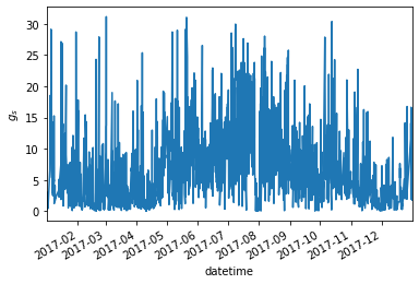
10.3.4.3.1. Distribution of observed \(g_s\)

gs_obs.plot()
plt.ylabel('$g_s$')

Text(0, 0.5, '$g_s$')

print('lai_max is {}'.format(lai_max))

lai_max is 5.0

10.3.4.4. Splitting the data to test and train

df_forcing_train, df_forcing_test, gs_train, gs_test = train_test_split(df_forcing, gs_obs, test_size=0.6, random_state=42)

kd=df_forcing_train.kdown
ta=df_forcing_train.Tair
rh=df_forcing_train.RH
pa=df_forcing_train.pres
smd=df_forcing_train.xsmd
lai=df_forcing_train.lai

10.3.4.5. Optimization

More info in here

10.3.4.5.1. Function to optimize

def fun_to_opts(G):
    [g1,g2, g3, g4, g5, g6]=[G[0],G[1],G[2],G[3],G[4],G[5]]
    gs_model,g_lai,g_kd,g_dq,g_ta,g_smd,g_z=cal_gs_mod(kd, ta, rh, pa, smd, lai,
                          [g1, g2, g3, g4, g5, g6],
                          g_max, lai_max, s1)
    gs_obs=gs_train
    o1=abs(1-np.std(gs_model)/np.std(gs_obs)) # normilized std difference
    o2=np.mean(abs(gs_model-gs_obs))/(np.mean(gs_obs))
    return [o1,o2],[gs_model.min()]

10.3.4.5.2. Problem definition and run

problem = Problem(6,2,1)
problem.types[0] = Real(.09, .5)
problem.types[1] = Real(100, 500)
problem.types[2] = Real(0, 1)
problem.types[3] = Real(0.4, 1)
problem.types[4] = Real(25, 55)
problem.types[5] = Real(0.02, 0.03)

problem.constraints[0] = ">=0"

problem.function = fun_to_opts
random.seed(12345)
algorithm=CMAES(problem, epsilons=[0.005])
algorithm.run(3000)

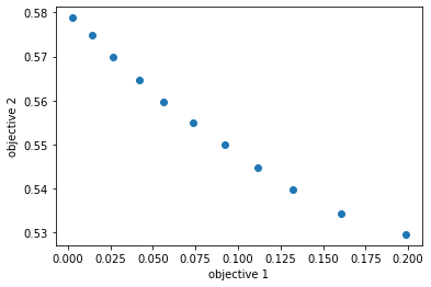
10.3.4.5.3. Solutions

print( " Obj1\t Obj2")

for solution in algorithm.result[:10]:
    print ("%0.3f\t%0.3f" % tuple(solution.objectives))

 Obj1    Obj2
0.073   0.555
0.112   0.545
0.161   0.534
0.056   0.560
0.003   0.579
0.092   0.550
0.199   0.530
0.133   0.540
0.026   0.570
0.014   0.575

f, ax = plt.subplots(1, 1)
plt.scatter([s.objectives[0] for s in algorithm.result],
           [s.objectives[1] for s in algorithm.result])
plt.xlabel('objective 1')
plt.ylabel('objective 2')

Text(0, 0.5, 'objective 2')

all_std=[s.objectives[0] for s in algorithm.result]
all_MAE=[s.objectives[1] for s in algorithm.result]
all_std=np.array(all_std)
all_MAE=np.array(all_MAE)

10.3.4.5.4. Choosing between : the median of two objectives, where obj1 is max or where obj2 is max

method='median' # 'obj1' or 'obj2' or 'median'
colors= ['b','g','r','y']

if method == 'median':
    idx_med=np.where(all_MAE==all_MAE[(all_std<=np.median(all_std))].min())[0][0]
elif method == 'obj1':
    idx_med=np.where(all_MAE==all_MAE[(all_std>=np.min(all_std))].max())[0][0]
elif method == 'obj2':
    idx_med=np.where(all_MAE==all_MAE[(all_std<=np.max(all_std))].min())[0][0]
print(all_std[idx_med])
print(all_MAE[idx_med])

0.07329333444496633
0.5549996145597578

[g1,g2,g3,g4,g5,g6] = algorithm.result[idx_med].variables

10.3.4.5.5. Saving the solution

with open('outputs/g1-g6/'+name+'-g1-g6.pkl','wb') as f:
    pickle.dump([g1,g2,g3,g4,g5,g6], f)

with open('outputs/g1-g6/'+name+'-g1-g6.pkl','rb') as f:
    [g1,g2,g3,g4,g5,g6]=pickle.load(f)

pd.DataFrame([np.round([g1,g2,g3,g4,g5,g6],3)],columns=['g1','g2','g3','g4','g5','g6'],index=[name])

	g1	g2	g3	g4	g5	g6
US-MMS	0.431	104.34	0.634	0.683	35.25	0.03

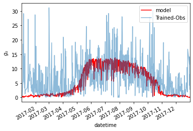
Let’s see how the model and observation compare for the training data set:

gs_model,g_lai,g_kd,g_dq,g_ta,g_smd,g_max=cal_gs_mod(kd, ta, rh, pa, smd, lai,
                          [g1, g2, g3, g4, g5, g6],
                          g_max, lai_max, s1)

gs_model.plot(color='r',label='model')
gs_train.plot(alpha=0.5,label='Trained-Obs')
plt.legend()
plt.ylabel('$g_s$')

Text(0, 0.5, '$g_s$')

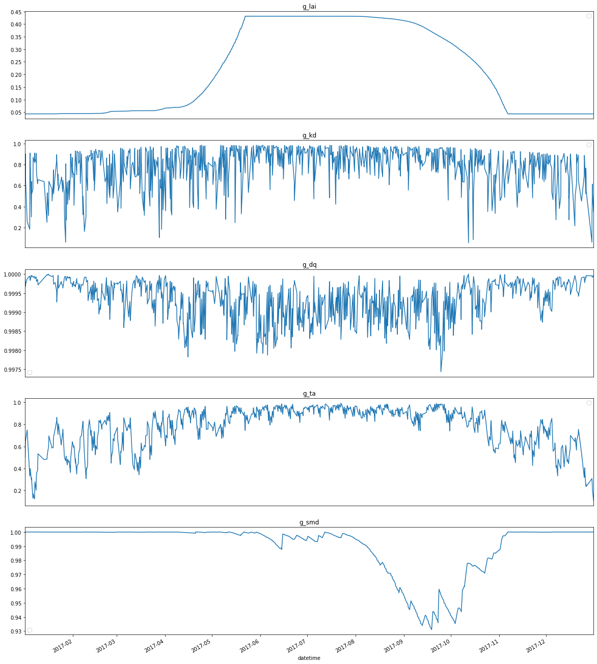
Let’s look at each individual \(g\) term:

g_dq=pd.DataFrame(g_dq,index=g_lai.index)
fig,axs=plt.subplots(5,1,figsize=(20,25))
a={'0':g_lai,'1':g_kd,'2':g_dq,'3':g_ta,'4':g_smd}
b={'0':'g_lai','1':'g_kd','2':'g_dq','3':'g_ta','4':'g_smd'}
for i in range(0,5):
    ax=axs[i]
    a[str(i)].plot(ax=ax)
    ax.set_title(b[str(i)])
    ax.legend('')
    if i!=4:
        ax.set_xticks([''])
        ax.set_xlabel('')

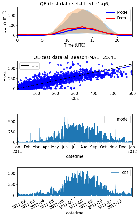
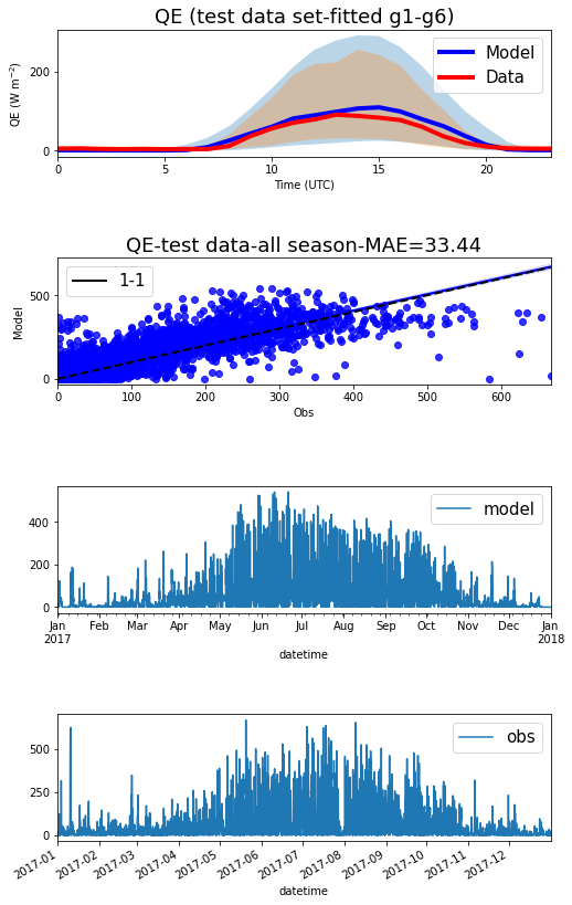
10.3.4.6. Running Supy with new g1-g6

alpha=2.6 # need to be tuned iteratively
name='US-MMS'
year=year
gs_plot_test(g1,g2,g3,g4,g5,g6,g_max,s1,name,year,alpha)

2020-03-26 10:38:44,539 — SuPy — INFO — All cache cleared.
2020-03-26 10:38:45,412 — SuPy — INFO — All cache cleared.
2020-03-26 10:38:47,776 — SuPy — INFO — ====================
2020-03-26 10:38:47,776 — SuPy — INFO — Simulation period:
2020-03-26 10:38:47,777 — SuPy — INFO —   Start: 2016-12-31 23:05:00
2020-03-26 10:38:47,778 — SuPy — INFO —   End: 2017-12-31 23:00:00
2020-03-26 10:38:47,779 — SuPy — INFO —
2020-03-26 10:38:47,780 — SuPy — INFO — No. of grids: 1
2020-03-26 10:38:47,782 — SuPy — INFO — SuPy is running in serial mode
2020-03-26 10:39:08,180 — SuPy — INFO — Execution time: 20.4 s
2020-03-26 10:39:08,181 — SuPy — INFO — ====================

g1=g1*alpha
g_max=g1*g_max
g1=1

g_max

37.03471400427182

10.3.4.7. Creating the table for all sites here (if more than one site is tuned)

sites=['US-MMS']
g1_g6_all=pd.DataFrame(columns=['g1','g2','g3','g4','g5','g6'])

for s in sites:
    with open('outputs/g1-g6/'+s+'-g1-g6.pkl','rb') as f:
        g1_g6_all.loc[s,:]=pickle.load(f)
g1_g6_all

	g1	g2	g3	g4	g5	g6
US-MMS	0.431336	104.34	0.633861	0.682953	35.25	0.0298504

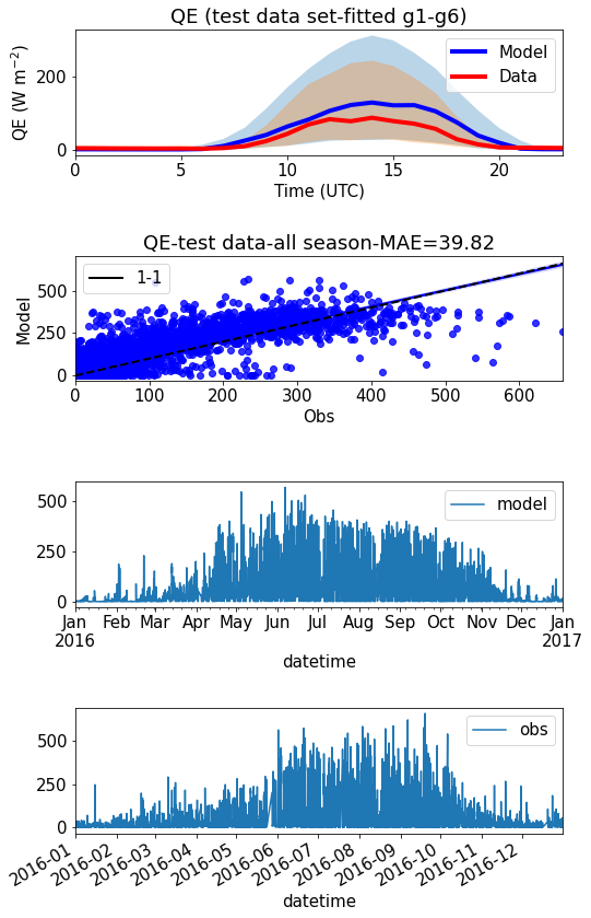
10.3.4.8. To test

10.3.4.8.1. US-MMS-2016

g1,g2,g3,g4,g5,g6=g1_g6_all.loc['US-MMS',:].values
g_max=g_max
g1=1
s1=5.56


name='US-MMS'
year=2016
df_forcing= read_forcing(name,year)
gs_plot_test(g1,g2,g3,g4,g5,g6,g_max,s1,name,year)

2020-03-26 10:41:58,297 — SuPy — INFO — All cache cleared.
2020-03-26 10:41:59,122 — SuPy — INFO — All cache cleared.
2020-03-26 10:42:01,787 — SuPy — INFO — ====================
2020-03-26 10:42:01,789 — SuPy — INFO — Simulation period:
2020-03-26 10:42:01,791 — SuPy — INFO —   Start: 2015-12-31 23:05:00
2020-03-26 10:42:01,801 — SuPy — INFO —   End: 2016-12-31 23:00:00
2020-03-26 10:42:01,802 — SuPy — INFO —
2020-03-26 10:42:01,807 — SuPy — INFO — No. of grids: 1
2020-03-26 10:42:01,810 — SuPy — INFO — SuPy is running in serial mode
2020-03-26 10:42:24,960 — SuPy — INFO — Execution time: 23.2 s
2020-03-26 10:42:24,961 — SuPy — INFO — ====================

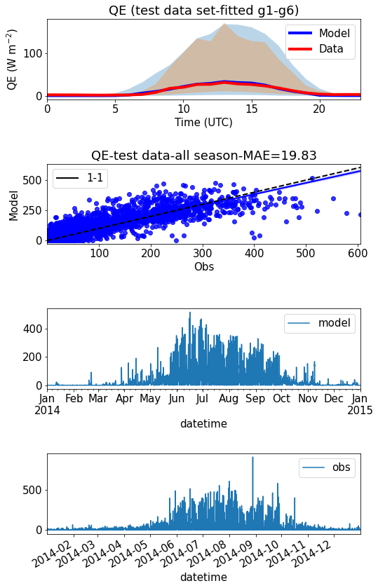
10.3.4.8.2. UMB-2014

g1,g2,g3,g4,g5,g6=g1_g6_all.loc['US-MMS',:].values
g_max=g_max
g1=1
s1=5.56

name='US-UMB'
year=2014
df_forcing= read_forcing(name,year)
gs_plot_test(g1,g2,g3,g4,g5,g6,g_max,s1,name,year)

2020-03-26 10:43:28,350 — SuPy — INFO — All cache cleared.
2020-03-26 10:43:29,145 — SuPy — INFO — All cache cleared.
2020-03-26 10:43:31,505 — SuPy — INFO — ====================
2020-03-26 10:43:31,506 — SuPy — INFO — Simulation period:
2020-03-26 10:43:31,506 — SuPy — INFO —   Start: 2013-12-31 23:05:00
2020-03-26 10:43:31,507 — SuPy — INFO —   End: 2014-12-31 23:00:00
2020-03-26 10:43:31,509 — SuPy — INFO —
2020-03-26 10:43:31,511 — SuPy — INFO — No. of grids: 1
2020-03-26 10:43:31,512 — SuPy — INFO — SuPy is running in serial mode
2020-03-26 10:43:45,433 — SuPy — INFO — Execution time: 13.9 s
2020-03-26 10:43:45,434 — SuPy — INFO — ====================

10.3.4.8.3. US-Oho-2011

g1,g2,g3,g4,g5,g6=g1_g6_all.loc['US-MMS',:].values
g_max=g_max
g1=1
s1=5.56

name='US-Oho'
year=2011
df_forcing= read_forcing(name,year)
gs_plot_test(g1,g2,g3,g4,g5,g6,g_max,s1,name,year)

2020-03-26 10:43:49,647 — SuPy — INFO — All cache cleared.
2020-03-26 10:43:50,493 — SuPy — INFO — All cache cleared.
2020-03-26 10:43:53,625 — SuPy — INFO — ====================
2020-03-26 10:43:53,626 — SuPy — INFO — Simulation period:
2020-03-26 10:43:53,627 — SuPy — INFO —   Start: 2010-12-31 23:05:00
2020-03-26 10:43:53,628 — SuPy — INFO —   End: 2011-12-31 23:00:00
2020-03-26 10:43:53,629 — SuPy — INFO —
2020-03-26 10:43:53,631 — SuPy — INFO — No. of grids: 1
2020-03-26 10:43:53,632 — SuPy — INFO — SuPy is running in serial mode
2020-03-26 10:44:11,821 — SuPy — INFO — Execution time: 18.2 s
2020-03-26 10:44:11,822 — SuPy — INFO — ====================